6 Checking Assumptions2
6.1 Checking Normality Assumptions
Shapiro-Wilk Test
The Shapiro-Wilk test tests the null hypothesis that the samples come from a normal distribution against the alternative hypothesis that the samples do not come from a normal distribution.
oneway_data[-1,] %>%
  rstatix::shapiro_test(Colorless,Pink,Orange,Green)
## # A tibble: 4 x 3
## variable statistic p
## <chr> <dbl> <dbl>
## 1 Colorless 0.913 0.499
## 2 Green 0.881 0.342
## 3 Orange 0.965 0.813
## 4 Pink 0.937 0.635shapiro.test(residuals(object = one_aov))##
## Shapiro-Wilk normality test
##
## data: residuals(object = one_aov)
## W = 0.92472, p-value = 0.1222QQ Plots
clean_oneway_data %>%
  mutate(Residual = one_aov$residuals) %>%
  ggplot(aes(sample = Residual)) +
  stat_qq() +
  stat_qq_line() +
  facet_wrap(~Type)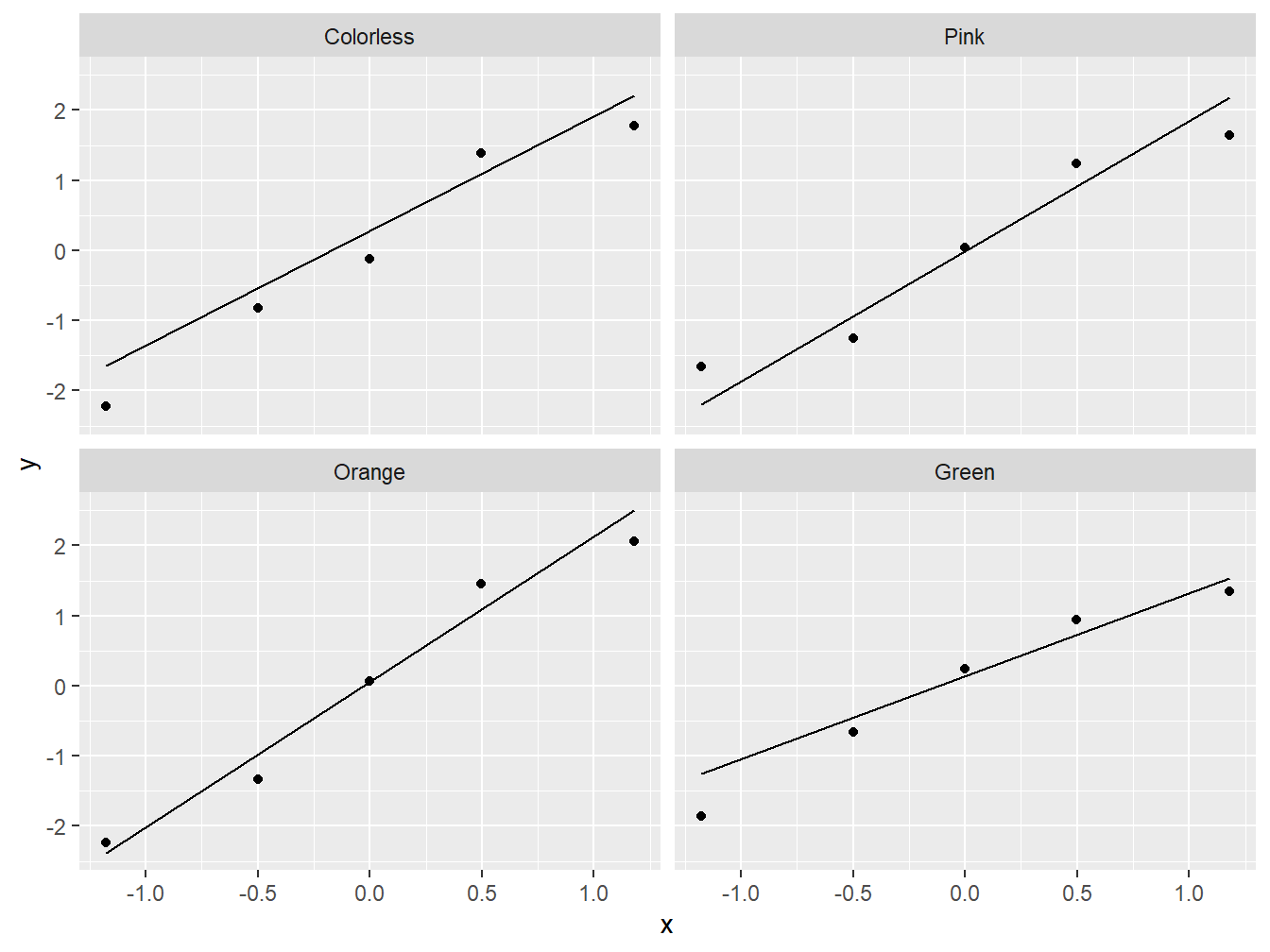
plot(one_aov,2)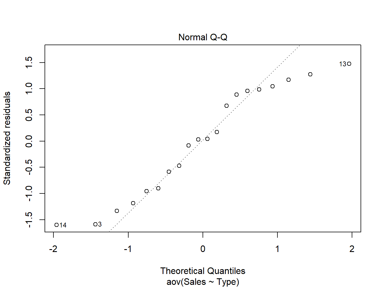
Histogram
clean_oneway_data %>%
  ggplot(aes(x = Sales)) +
  geom_histogram(bins = 30, color = "white") +
  geom_density() +
  facet_wrap(~Type)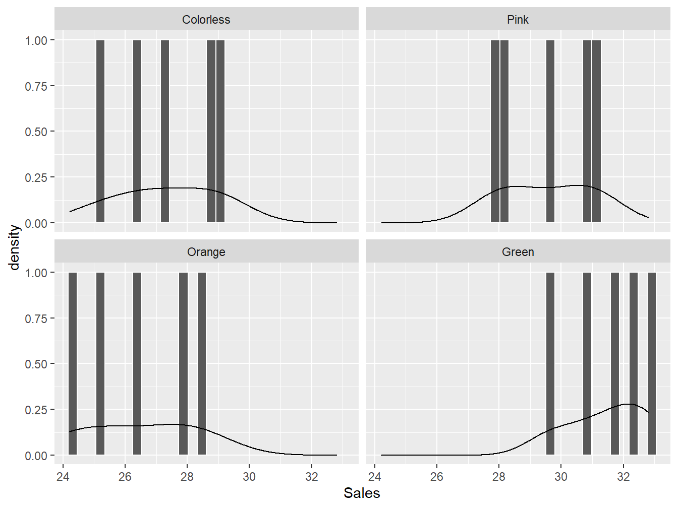
6.2 Checking Homogeneity of Variance Assumption
Bartlet’s Test
Bartlett’s test tests the null hypothesis that the group variances are equal against the alternative hypothesis that the group variances are not equal.
clean_oneway_data %>%
  bartlett.test(Sales ~ Type, data = .)
##
## Bartlett test of homogeneity of variances
##
## data: Sales by Type
## Bartlett's K-squared = 0.46564, df = 3, p-value = 0.9264clean_oneway_data %>%
ggboxplot(x = "Type", y = 'Sales',
fill = "Type",
palette = c("white", "pink", "orange", "green")) +
theme(legend.position = "none")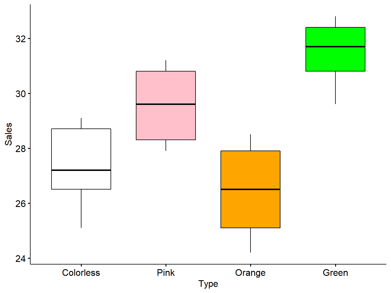 The variability within each group is represented by the vertical size of each box; i.e., the interquartile range (IQR). The boxplot shows that the variability is roughly equal for each group. Let’s look at some more ways to test the homogeneity of variance assumption.
Residual vs. Fitted Values Plot
plot(one_aov,1, las=1)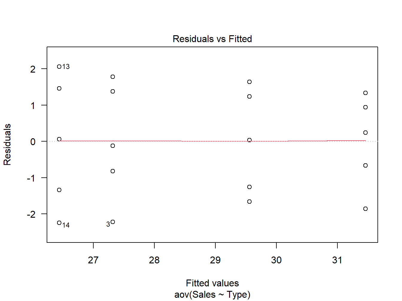 This plot shows the residuals (errors) on the y-axis and the fitted values (predicted values) on the x-axis. If the variance of each group is equal, the plot should show no pattern; in other words, the points should look like a cloud of random points. The plot shows that the variances are approximately homogenous since the residuals are distributed approximately equally above and below zero.
Standardised Residuals vs Fitted values Plot
plot(one_aov,3)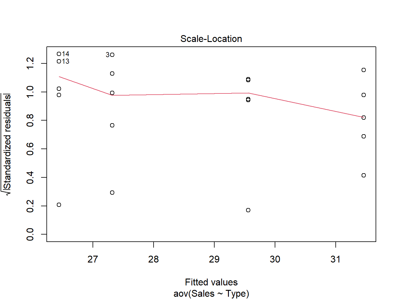
The more coincident the red line plot to the horizontal line at 1, the lesser possibility the violation of the homogeneity of variance assumption.